Continued from previous page

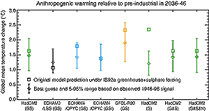
Figure 12.13: Global mean temperature in the decade 2036 to 2046
(relative to pre-industrial, in response to greenhouse gas and sulphate
aerosol forcing following the IS92a (IPCC, 1992) scenario), based on original
model simulations (squares) and after scaling to fit the observed signal
as in Figure 12.12(a) (diamonds), with 5 to
95% confidence intervals. While the original projections vary (depending,
for example, on each models climate sensitivity), the scale should
be independent of errors in both sensitivity and rate of oceanic heat uptake,
provided these errors are persistent over time. GS indicates combined greenhouse
and sulphate forcing. G shows the impact of setting the sulphate forcing
to zero but correcting the response to be consistent with observed 20th
century climate change. G&S indicates greenhouse and sulphate responses
estimated separately (in which case the result is also approximately independent,
under this forcing scenario, to persistent errors in the sulphate forcing
and response) and G&S&N indicates greenhouse, sulphate and natural
responses estimated separately (showing the small impact of natural forcing
on the diagnostic used for this analysis). (From Allen et al., 2000b.) |
Estimation of uncertainty in predictions
The scaling factors derived from optimal detection can also be used to constrain
predictions of future climate change resulting from anthropogenic emissions
(Allen et al., 2000b). The best guess scaling and uncertainty limits for each
component can be applied to the model predictions, providing objective uncertainty
limits that are based on observations. These estimates are independent of possible
errors in the individual models climate sensitivity and time-scale of
oceanic adjustment, provided these errors are persistent over time. An example
based on the IS92a (IPCC, 1992) GS scenario (whose exact forcing varies between
models, see Chapter 9, Table 9.1
for details) is shown in Figure 12.13 based on a limited
number of model simulations. Note that in each case, the original warming predicted
by the model lies in the range consistent with the observations. A rate of warming
of 0.1 to 0.2°C/decade is likely over the first few decades of the 21st
century under this scenario. Allen et al. (2000b) quote a 5 to 95% (very
likely) uncertainty range of 0.11 to 0.24°C/decade for the decades
1996 to 2046 under the IS92a scenario, but, given the uncertainties and assumptions
behind their analysis, the more cautious likely qualifier is used
here. For comparison, the simple model tuned to the results of seven AOGCMs
used for projections in Chapter 9 gives a range of 0.12
to 0.22°C/decade under the IS92a scenario, although it should be noted that
this similarity may reflect some cancellation of errors and equally good agreement
between the two approaches should not be expected for all scenarios, nor for
time-scales longer than the few decades for which the Allen et al. (2000b) approach
is valid. Figure 12.13 also shows that a similar range
of uncertainty is obtained if the greenhouse gas and sulphate components are
estimated separately, in which case the estimate of future warming for this
particular scenario is independent of possible errors in the amplitude of the
sulphate forcing and response. Most of the recent emission scenarios indicate
that future sulphate emissions will decrease rather than increase in the near
future. This would lead to a larger global warming since the greenhouse gas
component would no longer be reduced by sulphate forcing at the same rate as
in the past. The level of uncertainty also increases (see Allen et al., 2000b).
The final error bar in Figure 12.13 shows that including
the model-simulated response to natural forcing over the 20th century into the
analysis has little impact on the estimated anthropogenic warming in the 21st
century.
It must be stressed that the approach illustrated in Figure
12.13 only addresses the issue of uncertainty in the large-scale climate
response to a particular scenario of future greenhouse gas concentrations. This
is only one of many interlinked uncertainties in the climate projection problem,
as illustrated in Chapter 13, Figure
13.2. Research efforts to attach probabilities to climate projections and
scenarios are explored in Chapter 13, Section
13.5.2.3.
Forest et al. (2000) used simulations with an intermediate complexity climate
model in a related approach. They used optimal detection results following the
procedure of Allen and Tett (1999) to rule out combinations of model parameters
that yield simulations that are not consistent with observations. They find
that low values of the climate sensitivity (<1°C) are consistently ruled
out, but the upper bound on climate sensitivity and the rate of ocean heat uptake
remain very uncertain.
Other space-time approaches
North and Stevens (1998) use a space-frequency method that is closely related
to the space-time approach used in the studies discussed above (see Appendix
12.2). They analyse 100-year surface temperature time-series of grid box
mean surface temperatures in a global network of thirty six large (10°x10°)
grid boxes for greenhouse gas, sulphate aerosol, volcanic and solar cycle signals
in the frequency band with periods between about 8 and 17 years. The signal
patterns were derived from simulations with an EBM (see Section
12.2.3). The authors found highly significant responses to greenhouse gas,
sulphate aerosol, and volcanic forcing in the observations. Some uncertainty
in their conclusions arises from model uncertainty (see discussion in Section
12.2.3) and from the use of control simulations from older AOGCMs, which
had relatively low variability, for the estimation of internal climate variability.
A number of papers extend and analyse the North and Stevens (1998) approach.
Kim and Wu (2000) extend the methodology to data with higher (monthly) time
resolution and demonstrate that this may improve the detectability of climate
change signals. Leroy (1998) casts the results from North and Stevens (1998)
in a Bayesian framework. North and Wu (2001) modified the method to perform
space-time (rather than space-frequency) detection in the 100-year record. Their
results are broadly similar to those of Tett et al., (1999), Stott et al. (2001)
and North and Stevens (1998). However, their best guess includes a small sulphate
aerosol signal countered by a relatively small, but highly significant, greenhouse
gas signal.
All of the space-time and space-frequency optimal detection studies to date
indicate a discernible human influence on global climate and yield better-constrained
estimates of the magnitude of anthropogenic signals than approaches using spatial
information alone. In particular, the inclusion of temporal information can
reduce the degeneracy that may occur when more than one climate signal is included.
Thus, results from time-space methods generally detect anthropogenic signals
even if natural forcings are estimated simultaneously and show that the combination
of natural signals and internal variability is inconsistent with the observed
surface temperature record.
