Climate Change 2001: Mitigation

2.3.2 Quantitative Characteristics of Mitigation Scenarios

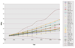
Figure 2.2: Global CO₂ emissions from baseline scenarios used for 550ppmv stabilization quantification (fossil fuel CO₂ emissions over the period 1990 to 2100 with the maximum and minimum numbers of the database of scenarios). This figure excludes the SRES scenarios (for legend details see Appendix 2.1).

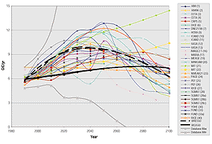
Figure 2.3: Global CO₂ emissions from mitigation scenarios for 550ppmv stabilization (fossil fuel CO₂ emissions over the period 1990 to 2100 with the maximum and minimum numbers of the database of scenarios). This figure excludes the post-SRES scenarios (for legend details see Appendix 2.1).

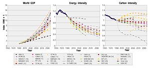
Figure 2.4: Range of baseline assumptions in GDP, energy intensity, and carbon intensity over the period 1990 to 2100 used for 550 ppmv stabilization analyses (indexed to 1990 levels), with historical trend data for comparison (for legend details see Appendix 2.1).

Figure 2.5: Scatter plot of GDP growth versus energy intensity reduction in baseline scenarios (including world and regional data).

From the large number of mitigation scenarios, a selection must be made in order to clarify in a manageable way the quantitative characteristics of mitigation scenarios. One of the efficient ways to analyze them is to focus on a typical mitigation target. As the most frequently studied mitigation target is the 550ppmv stabilization scenario, a total of 31 stabilization scenarios adopting that target were selected along with their baseline (reference or non-intervention) scenarios in order to analyze the characteristics of the stabilization scenarios as well as their baselines⁵. Figure 2.2 shows these baseline scenarios, and Figure 2.3 shows the mitigation scenarios for 550ppmv stabilization. (The sources and scenario names are noted in Appendix 2.1).

2.3.2.1 Characteristics of Baseline Scenarios

In order to analyze the characteristics of stabilization scenarios, it is very important to identify the features of the baseline scenarios that have been used for mitigation quantification. Although the general characteristics of non-intervention scenarios have already been analyzed in the SRES (Nakicenovic et al., 2000), more specific analyses are conducted here, focusing on the baseline scenarios that have been used for 550ppmv stabilization quantification.

First, it is clear that the range of CO₂ emissions in baseline scenarios used for 550ppmv stabilization quantification is very wide at the global level, as shown in Figure 2.2. The maximum levels of CO₂ emissions represent more than ten times the current levels, while the minimum level represents four times current levels. The range of baseline scenarios covers the upper half of the total range of the database, and most of them were estimated to be larger than IS92a (IPCC 1992 scenario “a”). This means that the baseline scenarios used for the 550ppmv stabilization analyses have a very wide range and are high relative to other studies.

This divergence can be explained by the Kaya identity (Kaya, 1990), which separates CO₂ emissions into three factors: gross domestic product (GDP), energy intensity, and carbon intensity⁶:

CO₂ emissions = GDP * Energy intensity * Carbon intensity = GDP * (energy/GDP) * (emissions/energy)

Figure 2.4 shows these factors. For comparability of the factors, which were not harmonized to be the same number among models in the base year of 1990, all the values are indexed to 1990 levels. CO₂ emissions are mostly determined by energy consumption. This, in turn, is determined by the levels of GDP, energy intensity, and carbon intensity. However, the ranges of GDP and of carbon intensities in the scenarios are larger than the range of energy intensities. This suggests that the large range of CO₂ emissions in the scenarios is primarily a reflection of the large ranges of GDP and carbon intensity in the scenarios. Thus, the assumptions made about economic growth and energy supply result in huge variations in CO₂ emission projections.

These characteristics are also observed in regional scenarios. For example, in both the OECD and non-OECD scenarios, CO₂, GDP, energy intensity, and carbon intensity have wide ranges, and in particular, the range among scenarios for the non-OECD nations is wider than the range among scenarios for OECD nations. In addition, the growth of CO₂ emissions in non-OECD nations is generally larger than the growth of emissions in OECD nations. This is mainly caused by higher GDP growth in the non-OECD countries.

With regard to regional comparisons, it is very difficult to come to any general conclusions, as the ranges involved in the regional scenarios are extraordinarily large. Moreover, with the exception of the USA, Europe, the Former Soviet Union (FSU) and China, the number of available scenarios is limited. However, some general trends can be identified that are associated with the medium ranges of the scenarios: for Asian countries, GDP growth is the most significant factor, resulting in high levels of energy use and CO₂ emissions; energy efficiency improvements are the most significant factor in the scenarios for China; and carbon intensity reductions are very high in Africa, Latin America, and Southeast Asia, because of drastic energy mix changes.

Other interesting characteristics at the global level can be identified in the relationships among GDP, energy intensity, and carbon intensity. Figure 2.5 shows a scatter plot of GDP growth rate versus energy intensity reduction from the baseline scenarios. As might be expected, the energy intensity reduction is higher with a higher GDP growth rate, while a lower energy intensity reduction is associated with a lower GDP growth rate. This relationship suggests that high economic growth scenarios assume high levels of progress in end-use technologies.

Unlike energy intensity reductions, carbon intensity reductions in the models are apparently seen as largely independent of economic growth and consequently are a function of societal choices, including energy and environmental policies. The scenarios do not show any clear relationship between energy intensity reduction and carbon intensity reduction. The values depend on regional characteristics in energy systems and technology combinations. Energy intensity reduction can include many measures other than fuel shifting. Most of the efficiency measures will result in lower carbon emissions, and fuel shifts from high-carbon to low- or non-carbon fuels can increase the efficiency of energy systems in many cases. However, carbon intensity reductions can also lead to reduced efficiency in energy systems, as in the case of shifts to biomass gasification or liquefaction, or result in increased energy consumption, as in the case of industrial carbon sequestration.

Box 2.3. Non-CO₂ Mitigation Scenarios

Since the publication of IPCC’s SAR, the literature on mitigation scenarios has continued to focus on the reduction of CO₂ emissions rather than on other GHGs. This is unfortunate because non-CO₂ emissions make up a significant fraction of the total “basket of gases” that must be reduced under the Kyoto Protocol. However, a small set of papers has reported on scenarios for mitigating non-CO₂ gases, especially CH₄ and N₂O. In one such paper, Reilly et al. (1999) compared scenarios for achieving emission reductions with and without non-CO₂ emissions in Annex B countries (those countries that are included in emission controls under the Kyoto Protocol). Scenarios that omitted measures for reducing non-CO₂ gases had 21% higher annual costs in 2010 than those that included them. Tuhkanen et al. (1999) and Lehtilä et al. (1999) came to similar conclusions — in a scenario analysis for 2010, they found that including CH₄ and N₂O in mitigation strategies for Finland reduced annual costs by 20% in the year 2010 relative to a baseline scenario. The general conclusion of these papers is that small reductions of GHG emissions, for example of the magnitude required by the Kyoto Protocol, can be accomplished at a lower cost by taking into account measures to reduce non-CO₂ gases, and that a small reduction of non-CO₂ gases can produce large impacts at low cost because of the high global warming potential (GWP) of these gases.

In another type of scenario analysis, Alcamo and Kreileman (1996) used the IMAGE 2 model to evaluate the environmental consequences of a large set of non-CO₂ and CO₂ mitigation scenarios. They concluded that non-CO₂ emissions would have to be controlled along with CO₂ emissions in order to slow the increase of atmospheric temperature to below prescribed levels. Hayhoe et al. (1999) pointed out two additional benefits of mitigating CH₄, an important non-CO₂ gas. First, most CH₄ reduction measures do not require the turnover of capital stock (as do CO₂ measures), and can therefore be carried out more rapidly than CO₂ reduction measures. Second, CH₄ reductions will have a more immediate impact on mitigating climate change than CO₂ reductions because the atmosphere responds more rapidly to changes in CH₄ than to CO₂ concentrations.

Other reports in this collection