A major advance since the SAR has been the increase in the range of techniques used to assess the quantitative agreement between observed and modelled climate change, and the evaluation of the degree to which the results are independent of the assumptions made in applying those techniques (Table 12.1). Also, some studies have based their conclusions on estimates of the amplitude of anthropogenic signals in the observations and consideration of their consistency with model projections. Estimates of the changes in forcing up to 1990 used in these studies, where available, are given in Table 12.2. In this section we assess new studies using a number of techniques, ranging from descriptive analyses of simple indices to sophisticated optimal detection techniques that incorporate the time and space-dependence of signals over the 20th century.
Table 12.1: Summary of the main detection and attribution studies considered. | |||||||||
Study | Signals | Signal source | Noise source | Method | S, V | Sources of uncertainty | Time-scale | No. of patterns | Detect |
Santer et al., 1996 | G, GS, O etc. | Equilibrium / future LLNL, GFDL R15, HadCM2 | GFDL R15, HadCM2, ECHAM1 | F, Corr | V | Internal variability | 25 year Annual and seasonal | 1 | GSO |
Hegerl, 1996, 1997 | G, GS | Future ECHAM3, HadCM2 | GFDL R15, ECHAM1, HadCM2; observation | F, Pattern | S | Internal variability | 30, 50 years Annual and JJA | 1, 2 | G, GS, S |
Tett et al., 1996 | G, GS, GSO | Historical HadCM2 | HadCM2 | F, Corr | V | Internal variability | 35 years | 1 | GSO |
Hegerl et al., 2000 | G, GS, Vol, Sol | Future, ECHAM3, HadCM2 | ECHAM3, HadCM2 | F, Pattern | S | Internal variability; model uncertainty | 30, 50 years Annual and JJA | 1, 2 | GS, G, S (not all cases) |
Allen and Tett, 1999 | G, GS, GSO | Historical HadCM2 | HadCM2 | F, pattern | V | Internal variability | 35 years Annual | 1, 2 | GSO and also G |
Tett et al., 1999 Stott et al., 2001 |
G,GS, Sol, Vol | Historical HadCM2 | HadCM2 | Timespace | S | Internal variability, 2 solar signals | 50 years decadal and seasonal | 2 or more | G, GS, Sol (Vol) |
North and Stevens, 1998 Leroy, 1998 |
G, GS, Sol, Vol | Historical EBM | GFDL ECHAM1, EBM | Freq-Space | S | Internal variability | Annual and hemispheric summer | 4 | G, S, Vol |
North and Wu, 2001 | Same+Had CM2 | Timespace | Annual | G, Vol | |||||
Barnett et al., 1999 | G, GS, GSIO Sol+vol | Future ECHAM3, ECHAM4, HadCM2, GFDL R15 | ECHAM3, ECHAM4, HadCM2, GFDL R15 | F, Pattern | S | Observed sampling error, model uncertainty, internal variability | 50 years JJA trends | 2 | GS, G, S (S not all cases) |
Hill et al., 2001 | G, GSO,Sol | Historical HadCM2 | HadCM2 | F, pattern | V | Internal variability | 35 years annual | 3 | G |
Tett et al., 2000 | G,GSTI, GSTIO, Nat | Historical HadCM3 | HadCM3 | Timespace | S | Internal variability | 50, 100 years decadal | 2 or more | G, SIT, GSTIO and Nat |
F, pattern | V | Internal variability | 35 years, annual | 2 | GSTI | ||||
The columns contain the following information: Study: the main reference to the study. Signals: outlines the principal signals considered: G-greenhouse gases, S-sulphate aerosol direct effect, T-tropospheric ozone, I-sulphate aerosol indirect effect, O-stratospheric ozone, Sol-solar, Vol-volcanoes, Nat-solar and volcanoes. Signal source: “historical” indicates the signal is taken from a historical hindcast simulation, “future” indicates that the pattern is taken from a prediction. Noise source: origin of the noise estimates. Method: “F” means fixed spatial pattern, “corr” indicates a correlation study, “pattern” an optimal detection study. S, V: “V” indicates a vertical temperature pattern, “S” a horizontal temperature pattern. Sources of uncertainty: any additional uncertainties allowed for are indicated. Modelled internal variability is allowed for in all studies. Time-scale: the lengths of time interval considered. (JJA= June-July-August) No. of patterns: the number of patterns considered simultaneously. Detect: signals detected. |
We begin in Section 12.4.1 with a brief discussion of detection studies that use simple indices and time-series analyses. In Section 12.4.2 we discuss recent pattern correlation studies (see Table 12.1) that assess the similarity between observed and modelled climate changes. Pattern correlation studies were discussed extensively in the SAR, although subsequently they received some criticism. We therefore also consider the criticism and studies that have evaluated the performance of pattern correlation techniques. Optimal detection studies of various kinds are assessed in Section 12.4.3. We consider first studies that use a single fixed spatial signal pattern (Section 12.4.3.1) and then studies that simul-taneously incorporate more than one fixed signal pattern (Section 12.4.3.2). Finally, optimal detection studies that take into account temporal as well as spatial variations (so-called space-time techniques) are assessed in Section 12.4.3.3.
Table 12.2: Estimated forcing from pre-industrial period to 1990 in simulations used in detection studies (Wm-2). GS indicates only direct sulphate forcing included, GSI indicates both direct and indirect effects included. Other details of the detection studies are given in Table 12.1. Details of the models are given in Chapter 8, Table 8.1. | |||||
Model | Aerosol | Baseline forcing | 1990 aerosol forcing | 1990 greenhouse gas forcing | Source of estimate |
HadCM2 | GS | 1760 | -0.6 | 1.9 | Mitchell and Johns, 1997 |
HadCM3 | GSI | 1860 | -1.0 | 2.0 | Tett et al., 2000 |
ECHAM3/LSG | GS | 1880 | -0.7 | 1.7 | Roeckner |
ECHAM4/OPYC | GSI | 1760 | -0.9 | 2.2 | Roeckner et al., 1999 |
GFDL_R30 | GS | 1760 | -0.6 | 2.1 | Stouffer |
CGCM1,2 | GS | 1760 | ~ -1.0 | ~2.2 | Boer et al., 2000a,b |
We provide various aids to the reader to clarify the distinction between the various detection and attribution techniques that have been used. Box 12.1 in Section 12.4.3 provides a simple intuitive description of optimal detection. Appendix 12.1 provides a more technical description and relates optimal detection to general linear regression. The differences between fixed pattern, space-time and space-frequency optimal detection methods are detailed in Appendix 12.2 and the relationship between pattern correlation and optimal detection methods is discussed in Appendix 12.3. Dimension reduction, a necessary part of optimal detection studies, is discussed in Appendix 12.4.
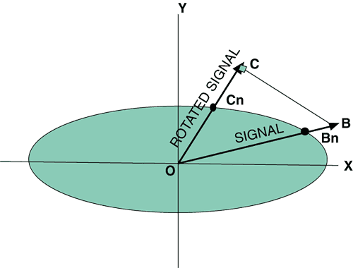
Box 12.1: Optimal detection
Optimal detection is a technique that may help to provide a clearer separation of a climate change fingerprint from natural internal climate variations. The principle is sketched in Figure 12.B1, below (after Hasselmann, 1976). Suppose for simplicity that most of the natural variability can be described in terms of two modes (well-defined spatial patterns) of variability. In the absence of climate change, the amplitudes of these two modes, plotted on a 2D diagram along OX and OY will vary with time, and for a given fraction of occasions (usually chosen as 95%), the amplitude of each mode will lie within the shaded ellipse. Suppose we are attempting to detect a fingerprint that can be made up of a linear combination of the two patterns such that it lies along OB. The signal to noise ratio is given by OB/OBn. Because our signal lies close to the direction of the main component of variability, the signal to noise ratio is small. On the other hand, we can choose a direction OC that overlaps less with the main component of natural variability such that the signal to noise ratio OC/OCn for the component of the signal that lies in direction OC is larger even though the projected signal OC is smaller then the full signal OB. Optimal detection techniques merely choose the direction OC that maximises the signal to noise ratio. This is equivalent to general linear regression (see Appendix 12.1). A good estimate of natural internal variability is required to optimise effectively. |
Other reports in this collection |