8.6.2 Coupled Model Variability
8.6.2.1 Comparison with the instrumental record
 
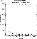
Figure 8.17: (a) Partial eigenvalue spectrum for the EOFs from eleven
CMIP AOGCMs. The observations (heavy line), together with their 95% confidence
limits (vertical bars), are obtained by projecting the observed surface
air temperature (Jones and Briffa, 1992; Rayner et al., 1996) onto the common
EOFs obtained from eleven CMIP AOGCMs. (b) as in (a) except for ten separate
100-year segments of the GFDL control run. Taken from Barnett (1999). |
Barnett (1999) concatenated the annual mean near-surface
temperature anomaly fields from the first 100 years of integration of eleven
CMIP control experiments to produce common empirical orthogonal functions (EOFs)
for the eleven AOGCMs. By projecting the Global Sea Ice and Sea Surface Temperature
(GISST) annual mean temperature anomaly data set (Rayner et al. 1996) onto these
common EOFs, he was able to estimate to what extent model variability represented
the observed variability. An analysis of the partial eigenvalue spectrum for
the different models (Figure 8.17a) suggests that there
is considerable disparity between the estimates of variability within the coupled
models. Some of this disparity arises from model drift and other low-frequency
variability. Intra-model disparity was much lower than inter-model disparity
as demonstrated by a similar common EOF analysis obtained from ten 100 year
segments in the 1,000 year GFDL_R15_a control run (Figure
8.17b). While the highest two modes were substantially underestimated in
the GFDL_R15_a model, the higher modes agreed better with observations. Error
bars on the observational data are large and when this is taken into account,
model disagreement with observations may not be significant. As Barnett (1999)
did not remove the trend over the 20th century in the GISST data set, the observations
also contain responses to both natural and anthropogenic forcing. One would
therefore expect control integrations from coupled climate models to underestimate
the observed spectrum at low frequencies (e.g., Folland et al., 1999).
An analogous study by Stouffer et al. (2000) compared the surface air temperature
variability from three long 1,000-year CMIP integrations (GFDL_R15_a, HadCM2,
ECHAM3/LSG (Large-Scale Geostrophic ocean model)) to the variability found in
the same observational data set (Jones and Briffa, 1992; Jones 1994). They argued
that, over the instrumental period, the simulated variability on annual to decadal
time-scales was fairly realistic both in terms of the geographical distribution
and the global mean values with a notable exception of the poor simulation of
observed tropical Pacific variability (Figure 8.18). The
HadCM2 model substantially overestimated tropical Pacific variability, whereas
it was underestimated in the GFDL_R15_a and ECHAM3/LSG models. They also noticed
that on the inter-decadal time-scale, the greatest variance in the models was
generally located near sea-ice margins close to regions of deep oceanic convection
and associated with low-frequency variations of the thermohaline circulation.
While the three models generally agreed on the dominant modes of variability,
there was substantial inter-model disparity in the magnitude of each mode. The
analysis of Stouffer et al. (2000) can easily be reconciled with Barnett (1999)
by realising that Stouffer et al. (2000) examined a subset (GFDL_R15_a, HadCM2,
ECHAM3/LSG models) of those CMIP models considered by Barnett (1999) that did
not experience climate drift, and that less emphasis was placed on the poor
resolution of tropical Pacific variability.
As an extension to the above analysis, Bell et al. (2000) compared annual mean
surface air temperature variability in sixteen CMIP control simulations to the
thermometer record, on time-scales of 1 year to 40 years (Figure
8.19). The authors found that: (1) thirteen of the sixteen CMIP models underestimate
variability in surface air temperatures over the global oceans; (2) twelve of
the sixteen models overestimate variability over land; (3) all the models overestimate
the ratio of air temperature variability over land to variability over oceans.
These results likely reflect problems in both the ocean and land-surface components
of climate models. In particular, underestimation of variability over oceans
may be due, at least in part, to weak or absent representations of El Niño
in the models; overestimation of variability over land may be due to poor land
surface parametrizations including insufficient soil moisture.
Duffy et al. (2000) also partitioned the CMIP models into those that are flux
adjusted and those that are not. They defined two measures of temperature variability
and applied them to the CMIP control simulations. The simulations differed substantially
in the amount of temperature variability they showed. However, on time-scales
of 1 year to 20 years, the flux adjusted simulations did not have significantly
less variability than the non-flux adjusted simulations; there is some suggestion
that they may have more variability. Thus it cannot be argued, for example,
that the use of flux adjusted models in studies of detection of anthropogenic
climate change tends to make observed temperature changes seem more significant
than they should be, compared to natural internal climate variability. Nevertheless,
it is still an open question as to how coupled model variability depends on
internal model parameters and resolution.

Figure 8.18: Power spectra of the detrended globally averaged
annual mean surface air temperature (SAT) anomaly. The curves represent
the estimates obtained from HadCM2 (blue), GFDL_R15_a (green) and
ECHAM3/LSG (red). The observed (black line) is from the globally averaged
annual mean SAT anomalies compiled by Jones and Briffa (1992). The
spectra are smoothed Fourier transforms of the autocovariance function
using a Tukey window of 100 lags for the models and 30 lags for the
observations. The two vertical lines represent the range of 95% confidence
in the spectral estimates for the model and the observations. Taken
from Stouffer et al. (2000). |
|

Figure 8.19: Simulated variability of annual mean surface air
temperatures over the last 40 years, 1959 to 1998 in sixteen CMIP
simulations and in observations (Jones, 1994; Parker et al., 1995).
(a) Global-mean temperature variability; four models show higher than
observed amounts of variability. (b) Mean over-ocean temperature variability;
three models show higher than observed amounts of variability. (c)
Mean over-land temperature variability; four models show less than
observed amounts of variability. (d) Ratio of over-land to over-ocean
temperature variability; all models show higher than observed ratios.
Taken from Bell et al. (2000). |
|
8.6.2.2 Comparison with palaeo-data
There have been relatively few studies which have undertaken a systematic comparison
of AOGCM variability with variability found in the Holocene proxy temperature
record. However, three studies (from the MPI (Max Planck Institute), Hadley
Centre and GFDL) that focus on the analysis of long control integrations are
available. Barnett et al. (1996) demonstrated that the GFDL_R15_a (Stouffer
et al., 1994) and ECHAM1/LSG (Cubasch et al., 1994) models underestimate the
levels of decadal-scale variability in summer palaeo-temperature proxies from
1600 to 1950 (expanded version of Bradley and Jones, 1993), with increasing
disparity with observations at lower frequencies.
Using annual and decadal mean near-surface palaeo-temperature reconstructions
at seventeen locations Jones et al. (1998) demonstrated, through a principal
component analysis, that the standard deviation of the GFDL_R15_a model (Stouffer
et al., 1994) and the HadCM2 model (Johns et al., 1997; Tett et al., 1997) principal
component time-series compared favourably with both proxy and observed data.
Time-series of the top seven principal components did, however, show much less
century time-scale variability than in the proxy time-series. This was especially
true in the HadCM2 model that was dominated by tropic-wide decadal variability.
Through cross-spectral analysis they concluded that the GFDL control integration
bears a remarkable similarity in its statistical properties to that obtained
from the proxy data. In view of this similarity it appears the spatial structures
from the control integration can be used to represent the spatial structures
of naturally occurring variations in near-surface air temperature. This
conclusion was also highlighted by Delworth and Mann (2000) who noted that both
palaeo-temperature reconstructions (Mann et al., 1998) and the GFDL_R15_a coupled
model suggest a distinct oscillatory mode of climate variability (with an approximate
time-scale of about 70 years) of hemispheric scale and centred around the North
Atlantic.


