This "global warming" thing... what Watt is what?
JunkScience.com
Updated August 2007
archive.com/ipcc_tar/ and changed primary TAR links to point to this resource This resource was mirrored from pame.arctic-council.org/climate/ipcc_tar/ by HTTrack Website Copier/3.x [XR&CO'2006], Mon, 30 Oct 2006 06:27:44 GMT.Note: this page uses Greek characters which may not display correctly depending on the code page available on the user's system. If you receive spurious characters this may help you try to sort it out: in order of use -- Δ: Delta, α: alpha, σ: sigma, λ: lambda and π: pi are used to signify change, the CO2 conversion constant 5.35, the Stefan-Boltzmann constant, about 0.5 K/Wm-2 and the value 3.14159 respectively. In addition to these the symbols °: degree, ±: +/- (plus or minus) and ≈: asymptotic to (almost equal to) are used.
Note also: The IPCC TAR host sites have an unfortunate tendency to become unavailable without notice so we are posting double links to both a primary and mirror site. If this does not resolve the issue we'll establish our own mirror.
Update January 2008: As the IPCC Third Assessment Report sites are being removed we have activated a local mirror http://www.junkscience
Preamble:
Global political and media attention are focused to the point of obsession on potential climate changes resulting from a doubling of atmospheric carbon dioxide (CO2). There is nothing particularly significant about this arbitrary figure other than it having caught the imagination of many, probably because it's a simple concept, oft repeated. Given this obsession we, too, will base our calculations on the doubling of this trace gas in the atmosphere.
In this document we are concentrating on global mean temperature although there is no evidence this is a particularly useful metric. Moreover, the focus is on radiative forcing, specifically from a doubling of atmospheric carbon dioxide (2xCO2), even though transport (convective adjustment) is of far greater significance. Any effect on this transport by slight greenhouse enhancement is as yet poorly understood. This is highly significant because, if Earth's surface cooled by radiation alone, (that is, in the absence of convective adjustment), surface temperatures would average 350 K (Möller and Manabe, 1961) rather than about 288 K, as they do now.
In global warming and climate studies, figures are often given in Watts per meter squared (
Before we begin let us note that there have been many excellent researchers who have pointed out that the concept of a globally averaged forcing constant is flawed and they are right. Sensitivity absolutely depends on where the forcing is applied and when. Unfortunately a globally averaged forcing value is applied via climate models and cited in IPCC documents and we are thus stuck with addressing an invalid value in common use.
Additionally, climate models make much of water vapor "feedbacks" -- a multiplier effect due to a small warming from carbon dioxide increasing evaporation and thus adding to the major greenhouse gas, water vapor -- this in turn is supposed to increase the greenhouse effect, leading to more evaporation and yet more warming and so on.
The amount of water vapor in the atmosphere is not a simple function of evaporation, however. All of the water vapor that is being continuously evaporated from the Earth's surface must eventually return to the surface as precipitation. The climate system strikes a balance, allowing only so much water vapor to accumulate before it is depleted by either rain or snow.
The term used to describe this self-limiting process is "precipitation efficiency," which is a measure of how readily precipitation processes in clouds convert cloud water into droplets large enough to fall to the surface. Theoretical research has shown that for a given amount of sunlight, high precipitation efficiency leads to cool, dry climates and low precipitation efficiency leads to warm, moist climates. (Rennó, 1994)
Within the restrictive parameters of political and media focus and with the somewhat skewed outlook of contemporary climate models then, let us follow the
numbers and see where they lead.
Key Points:
|
Estimated forcing from 2xCO2:
The IPCC (alt: IPCC) and the European Environment Agency both provide the formula for calculating change in radiative forcing (ΔF) in Wm-2. For carbon dioxide (CO2) this formula is given as ΔF = αln(C/Co) where C and Co are the current and pre-industrial concentrations of CO2, respectively and α = 5.35. Some would immediately argue this overstates average net forcing from increasing atmospheric CO2 and we'd tend to agree but the inflated value is not important, at least, not yet -- call it an inbuilt "safety margin," if you like.
Atmospheric CO2 is presented in parts per million by volume (ppmv). There is no universal standard for what we mean by a doubling of CO2 and various numbers are used, most commonly 560 (2x280 -- the common pre-Industrial revolution reference) and 600 (2x300 -- presumably benchmarked from early in the Twentieth Century).
Since most people seem to conceive the situation as two times "natural," which we take to mean immediately pre-Industrial Revolution, we'll be
using the former. From the above formula then, the change in forcing from a doubling of pre-Industrial Revolution atmospheric CO2 =
According to the National Academies' Climate Change Science: An Analysis of Some Key Questions (2001), doubling CO2 (to 600 ppmv) would lead to a forcing of about 4 W/m2, so we guess these figures are close enough for our purposes here.
How much warming is that?
What does this 3.7 Wm-2 mean? How much warming does that equate to for the planet's surface?
The IPCC gives a fairly large range of estimated warming, with references scattered through the TAR (Third Assessment Report) varying by up to 500% and are thus not particularly helpful. In fact, between the SAR and TAR (second and third reports) there's everything from a fraction of a degree to a one-to-one ratio Watts to degrees. Let's try to estimate it by other means.
Calculating using the Stefan-Boltzmann Constant:
|
|
If we use Stefan's Constant to derive greenhouse in Wm-2 as in the following:
G = σ(Ts4 - Te4) = σTs4 - OLR = 390.11 - 239.76 = 150.35 Wm-2 where G is the
global average greenhouse effect, σ is the Stefan-Boltzmann Constant, Ts = 288 K, Te = 255 K and OLR signifies Outgoing Longwave
Radiation, we have a figure of 150.35 Wm-2 and net warming of 33 °C, thus as a linear relationship a ΔF of 1 Wm-2 ≈ 0.22 °C.
Implied then is an increase of 0.81 °C from ΔF 3.7 Wm-2, the value estimated for a doubling of atmospheric carbon dioxide.
Alternatively, working back from our calculated 390.1 Wm-2 above (from net temperature) + ΔF 3.7 Wm-2 (the value estimated for a doubling of atmospheric carbon dioxide), we get (393.8/σ)1/4, yielding 288.68 K for a net warming of 0.68 °C, so ΔF of 1 Wm-2 ≈ 0.18 °C.
Both our figures derived so far are much smaller than frequently cited estimates for warming from a doubling of pre-Industrial Revolution atmospheric carbon dioxide.
Sidebar:There is a school of thought that 255 K is too low a value for a greenhouse-free world since this value is calculated with albedo (reflection of incoming
solar radiation) from clouds and atmospheric backscatter included.
|
Let's try some other methods.
Calculating using Kiehl and Trenberth's Global Mean Energy Budget:
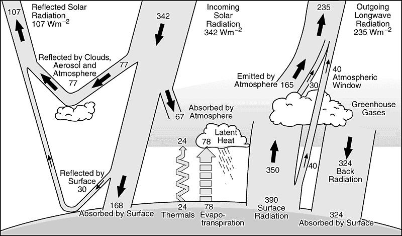 This graphic is
from Earth’s Annual Global Mean Energy Budget (Kiehl and Trenberth, 1997). "Back radiation" (downwelling
longwave radiation from the atmosphere) is listed twice as high as our calculated value at 324 Wm-2 (this is as derived by climate models for
attribution purposes -- see the linked paper for details).
This graphic is
from Earth’s Annual Global Mean Energy Budget (Kiehl and Trenberth, 1997). "Back radiation" (downwelling
longwave radiation from the atmosphere) is listed twice as high as our calculated value at 324 Wm-2 (this is as derived by climate models for
attribution purposes -- see the linked paper for details).
On the assumption that this represents Earth's greenhouse effect from all sources we can simply divide the estimate of Earth's greenhouse effect of 32 or 33 °C, (depending on whether Earth "should" be 287 or 288 K (roughly 14 or 15 °C) for a mean temperature) by the number of Watts.
If we split the difference we get 32.5/324 or 1 Wm-2 ≈ 0.1 °C. This means the ΔF 3.7 Wm-2 from increased CO2 would result in 0.37 °C warming in total.
That would be neat, simple and convenient, although it is only about half our calculated value -- but is it a reasonable rule of thumb? We've gone from small to insignificant as far as warming from added carbon dioxide goes and that certainly isn't how the story's been told.
Sidebar:Earth's mean temperature is believed to be between those two figures of 14 and 15 °C, so it's either a little bit warm or a little bit cool these days but never mind. The Elusive Absolute Surface Air Temperature (SAT) is supposed to be available by summing the current anomaly with 14.0 °C (287.15 K), according to GISS that would be 0.63 for the Jan-Dec average 2005, so 14.63 °C (287.78 K) for the global mean for 2005. |
Support in the literature for such low sensitivity -- the seminal work of Sherwood B. Idso:
In CO2-induced global warming: a skeptic’s view of potential climate change, 1998, Idso describes no less than eight natural experiments from which he derived surface air temperature sensitivity factors ≈ 0.17 °C/Wm-2 inland and ≈ 0.09 °C/Wm-2 by the coast. For the polar regions he derives a figure of ≈ 0.2 °C/Wm-2 and for all other regions ≈ 0.09 °C/Wm-2 for a global mean of ≈ 0.1 °C/Wm-2.
Significantly, Idso derived sensitivity figures in agreement for the world as we find it today at local, regional and planetary scales, over billions of
years of the planet's history and over our nearest celestial neighbors. Finding a relationship that holds over such physical and temporal scales to be mere
coincidence is unlikely, to say the least, and thus inspires some confidence in the global mean value of ≈ 0.1 °C/Wm-2.
|
The implications of Idso's research are the same as previously stated for our calculation derived from Kiehl and Trenberth, above, at ≈ 0.1 °C/Wm-2 and so would result in 0.37 °C warming for a doubling of atmospheric carbon dioxide. |
Is the world still responding that way or is the greenhouse effect accelerating?
We need to try calculating this yet another way to see if we come up with similar numbers. What we really need is something at or near the current temperature range because the temperature response may be non-linear or unduly influenced by anthropogenic effects.
Calculating using Roger Pielke, Sr.'s derivation from IPCC forcing tables and contemporary warming:
The IPCC's estimate of additional forcing from all added CO2 since the Industrial Revolution is ≈ 1.5 Wm-2, the equivalent
of our ΔF above for a value of 370 ppmv. Over the same period they estimate net warming of 0.6
± 0.2 °C alt: 0.6 ± 0.2 °C
. Professor Roger Pielke, Sr., suggests a figure of 26.5-28% of contemporary warming is attributable
to atmospheric carbon dioxide by estimating from IPCC-supplied forcing tables. Of the IPCC's estimated
|
Implied by the IPCC's forcing estimates as extracted by Pielke is a ΔT of ≈ 0.4 °C from ΔF 3.7 Wm-2 from a doubling of atmospheric CO2. Now we have our original blackbody calculation of 0.7-0.8 °C warming from 2xCO2 and Kiehl and Trenberth's global energy budget, Idso's eight natural experiments and Pielke's derivation from the IPCC's forcing estimates all yielding 0.4 °C or less. |
Why are our numbers so low?
Perhaps there are some as yet unnamed or at least un-quantified negative forcings influencing the planet's temperature such that these direct divisions are only yielding about half the expected value.
There is no implied conflict with calculations using the Stefan-Boltzmann constant since the real-world measures are negative forcing-inclusive. That is, increases in cloud albedo from increased evaporation following a small warming, for example, are not included in straight S-B calculations but do perturb the world's measured response.
Suppose we allocate all estimated warming from start-of-record through 2000 to enhanced greenhouse, i.e., ΔF 2.4 Wm-2 from increased CO2 and the ubiquitous "other" greenhouse gases (GHGs). By claiming the portion allocated to solar and land-use change for enhanced greenhouse we remove all contention and presumably include all actual feedbacks (those really operating in the physical world).
ΔF 2.4 Wm-2 from increased CO2 and all other GHGs combined ≈ 0.6 °C, 1 Wm-2 ≈ 0.25 °C (close to our original calculation with CO2 for all forms greenhouse). ΔF 3.7 Wm-2 from increased CO2 would then be ≈ 0.93 °C.
Assuming a proportional increase in all GHGs, despite CH4 apparently having achieved atmospheric equilibrium, ΔF 6.3 Wm-2 still only extrapolates to total ΔT <1.6 °C (that is, +1 °C from current estimate).
Looking forward for the worst case scenario:That's worth repeating. Despite knowing the sun has become more active we allocate all estimated temperature change to GHGs, extrapolate forward all values to a potential doubling of atmospheric carbon dioxide and, using the real world response numbers to date, we still only come up with a total potential warming of <1.6 °C including that already experienced since the latter 1800s. |
Let's have a look at a few more of the numbers floating around out there:
From the NAS CCS Report:
According to the National Academies' Climate Change Science: An Analysis of Some Key Questions (2001): "If there were no climate feedbacks, the response of Earth's mean temperature to a forcing of 4 W/m2 (the forcing for a doubled atmospheric CO2) would be an increase of about 1.2 °C (about 2.2 °F)." Thus 0.3 °C per Wm-2.
This is not too far from our original calculation, although it would suggest current ΔF (all GHGs) should deliver ΔT 0.8 °C, at the very limit of estimated contemporary change and leaving no room for any other positive forcings. This suggests the conversion factor is too high. Nonetheless, implied is a ΔT of 1.1 °C from ΔF 3.7 Wm-2 from increased CO2 (we've already experienced at least half that since the Industrial Revolution).
Huang's analysis of Crowley:
In Merging Information from Different Resources for New Insights into Climate Change in the Past and Future, Geophysical Research Letters, Vol. 31, L13205, 8 July 2004, Huang's analysis of the reconstructed temperature and radiative forcing [Crowley, 2000] series offers an independent estimate of the transient climate-forcing response rate of 0.4 - 0.7 K per Wm-2. Implied is a ΔT of 1.48 to 2.59 °C from ΔF 3.7 Wm-2 from doubled CO2 and current ΔF all GHGs of 2.4 Wm-2 should deliver between 0.96 and 1.68 °C ΔT. That is a rather long way from the Earth's demonstrated response to date (ΔF all GHGs 2.4 Wm-2 resulting in ΔT of 0.6 °C). Tentatively marked as somewhat dubious.
Climate models and the "Hansen Factor":
( Drawing from Reports to the Nation on Our Changing
Planet: Our Changing Climate, Fall 1997 issue [1.78Mb .pdf, 28pp], from NOAA's Office of Global Programs, now incorporated in the Climate Program Office (CPO).
)
This sounds like an impressive pedigree, doesn't it? Both Huang and Hansen provide figures of around three-fourths of a degree for every Watt per meter
squared. Looks like the rest of us are a long way out... or not.
HUMAN-MADE climate forcings, mainly greenhouse gases, heat the earth’s surface at a rate of about two watts per square meter—the equivalent of two
tiny one-watt bulbs burning over every square meter of the planet. The full effect of the warming is slowed by the ocean, because it can absorb so much heat.
The ocean’s surface begins to warm, but before it can heat up much, the surface water is mixed down and replaced by colder water from below. Scientists now
think it takes about a century for the ocean to approach its new temperature.
The implication is clear -- Earth should have warmed 1 - 2 °C under the influence of an added 2 Wm-2 from anthropogenic sources,
it's just hiding in the ocean. We'll revisit this.
According to the IPCC, global mean temperature rose 0.6 ± 0.2 °C from the late 19th Century through 2000. From the same source ΔF from
increased atmospheric carbon dioxide is calculated as +1.4 Wm-2, while the increase from all greenhouse gases combined is supposed to be 2.4 Wm-2.
Ignoring the much-argued about solar influence over the period and using the "Hansen Factor" of 0.75 °C per Wm-2, the world
should have warmed ≈ 1.8 °C from enhanced greenhouse forcing alone -- 2.4 °C if we use the model's 1:1 ratio. Obviously a simplistic
"greenhouse gas increase = n degrees warming" will not do since the real world has only delivered between one-sixth and one-third that value
with the greatest confidence being one-quarter (0.6 ± 0.2 or 0.4 to 0.8 °C). Definitely marked as dubious.
Looking at the problem another way -- maxing out Hansen's reduced ice age forcing of 6.6 ± 1.5 Wm-2 we get 8.1 Wm-2
for an observed ΔT of ≈ 5 °C. Presumably then 390.11 (from Stefan's constant, above) - 8.1 = 382 Wm-2 and this, according to
Hansen, should resolve to 288 - 5 = 283 K. However, (382/σ)1/4 yields 286.49 K, giving us a cooling not of 5 K but 1.5 K -- less than
one-third the expected value.
Working from temperature to derive the change in Wm-2, σ2834 = 363.71 Wm-2, which subtracted from 390.11 leaves us
26.4 Wm-2 rather than at most 8.1 as per Hansen. Why the shortfall? Perhaps there being no negative listing for solar in Hansen's ice age
forcings should have tipped us off. The Milankovitch theory attributing ice ages to changes in the eccentricity of the Earth's orbit with ~100Kyr periodicity is well subscribed. No model has
yet been able to fit orbital changes with our understanding of glacial and interglacial periods (glacial retreat occurring prior to increases in insolation...),
although changes in obliquity (41Kyr) and precession (23Kyr) do seem to work out more or less as anticipated. No calculation of change in insolation due to
Milankovitch cycles is offered here because they are an insufficient explanation for the onset of glacial/interglacial periods. That said, there are alternate hypotheses, such as Origin of the 100 Kyr Glacial Cycle: eccentricity or
orbital inclination? by Muller and MacDonald. Their work on orbital inclination certainly suggests much improved timing, at least and their pursuit of evidence of extraterrestrial accretion noteworthy. The implied increase in albedo, coupled with
a reduction in that most important of greenhouse gases, water vapor, offers a plausible feedback mechanism. It has the attractive although unproven addition of
a possible reason for the sudden onset of the ~100Kyr cycle (c.900Kyr ago) due to an injection of dust into the Solar System, possibly from the destruction of a
comet. So, ice ages and their cause(s) are as yet poorly understood but there are certainly plausible hypotheses to explain Hansen's marvelous, magical (and
missing) 20-odd Watts per meter squared. Note that would be the anticipated shortfall in steady-state forcing if Earth behaved as a perfect blackbody but is
less than half the required net change at Earth's apparent climate sensitivity -- the two are not claimed to be the same. Our calculations from Kiehl and Trenberth, along with those of both Idso and Pielke, indicate direct calculation using the Stefan-Boltzmann constant
overstates climate sensitivity by a factor of 2 by omitting the Earth's natural negative feedback mechanisms. In turn, Hansen overstates S-B-derived figures by
a factor of more than 3. The conclusion here is that the "Hansen Factor" is then at least 3 times too large and probably 6-8 times.
Going by the IPCC (alt: IPCC),
not very well at all. Here's the LOSU index (LOSU = level of scientific understanding):
It would perhaps be fairest to say we have a "limited understanding" of how the atmosphere and climate forcing works. From our results above it
appears there's large disagreement between empirical measures and models' expectations.
From the Third Assessment Report (alt: Third Assessment Report) again:
"The climate sensitivity parameter (global mean surface temperature response ΔTs to the radiative forcing ΔF) is defined as: ΔTs
/ ΔF = λ. In the one-dimensional radiative-convective models, wherein the concept was first initiated, λ is a nearly invariant parameter, typically, about
0.5 K/Wm-2. Although the value of the parameter “λ” can vary from one model to another, within each model it is found to be remarkably constant
for a wide range of radiative perturbations. The invariance of has made the radiative forcing concept appealing as a convenient measure to estimate the global,
annual mean surface temperature response, without taking the recourse to actually run and analyse, say, a three-dimensional atmosphere-ocean general circulation
model (AOGCM) simulation."
"Overall, the three-dimensional AOGCM experiments performed thus far show that the radiative forcing continues to serve as a good estimator for the
global mean surface temperature response but not to a quantitatively rigorous extent as in the case of the one-dimensional radiative-convective models. Several
GCM studies suggest a similar global mean climate sensitivity for the spatially homogeneous and for many but not all of the spatially inhomogeneous forcings of
relevance for climate change in the industrial era. Paleoclimate simulations also suggest the idea of similarities in climate sensitivity for a spatially
homogeneous and an inhomogeneous forcing (arising due to the presence of continental ice sheets at mid- to high northern latitudes during the last glacial
maximum). However, different values of climate sensitivity can result from the different GCMs which, in turn, are different from the λ values obtained with the
radiative-convective models. ...
However, in a general sense and considering arbitrary forcing types, the variation in λ could be substantially higher (50% or more) and the climate response
much more complex (Hansen et al., 1997a). It is noted that the climate sensitivity for some of the forcings that have
potentially occurred in the industrial era have yet to be comprehensively investigated."
"Another important limitation of the concept is that there are parameters other than global mean surface temperature that need to be determined, and
that are as important from a climate and societal impacts perspective; the forcing concept cannot provide estimates for such climate parameters as directly as
for the global mean surface temperature response. There has been considerably less research on the relationship of the equilibrium response in such parameters
as precipitation, ice extent, sea level, etc., to the imposed radiative forcing."
In modelers' own words, not very well: Principal Model Deficiencies
ModelE [2006] compares the atmospheric model climatology with observations. Model shortcomings include ~25% regional deficiency of summer stratus cloud
cover off the west coast of the continents with resulting excessive absorption of solar radiation by as much as 50 W/m2, deficiency in absorbed solar radiation
and net radiation over other tropical regions by typically 20 W/m2, sea level pressure too high by 4-8 hPa in the winter in the Arctic and 2-4 hPa too low in
all seasons in the tropics, ~20% deficiency of rainfall over the Amazon basin, ~25% deficiency in summer cloud cover in the western United States and central
Asia with a corresponding ~5°C excessive summer warmth in these regions. In addition to the inaccuracies in the simulated climatology, another shortcoming
of the atmospheric model for climate change studies is the absence of a gravity wave representation, as noted above, which may affect the nature of interactions
between the troposphere and stratosphere. The stratospheric variability is less than observed, as shown by analysis of the present 20-layer 4°x5° atmospheric
model by J. Perlwitz [personal communication]. In a 50-year control run Perlwitz finds that the interannual variability of seasonal mean temperature in the
stratosphere maximizes in the region of the subpolar jet streams at realistic values, but the model produces only six sudden stratospheric warmings (SSWs) in 50
years, compared with about one every two years in the real world. ... Climate
simulations for 1880-2003 with GISS modelE There is nothing particularly egregious here, save perhaps this is identical to the deficiency statement of papers 2 years prior despite the massive funding
expended on maintaining and running these video games. Models do not handle clouds and moisture at all well yet and NASA's Goddard Institute for Space Studies'
pride and joy is no exception. Placing excessive trust in the models, however, is not a recommended procedure.
In Earth's Energy Imbalance: Confirmation and Implications Hansen, et al, state: Our climate model,
driven mainly by increasing human-made greenhouse gases and aerosols, among other forcings, calculates that Earth is now absorbing 0.85 ± 0.15 watts per square
meter more energy from the Sun than it is emitting to space. This imbalance is confirmed by precise measurements of increasing ocean heat content over the past
10 years.
When that paper was written the model output was a fair wiggle-fit with Willis (2004) and Levitus
(2004).
So, Hansen's model is dumping heat into the oceans at roughly 0.8 Wm-2 and the bulk ocean heat rise mid-1993 - mid-2003 sort of matched that
-- if only the world would remain constant and conform to the models we'd have this "global warming" thing sorted. Like all happy accidents, however,
this good thing came to an end, too.
Lyman et al (2006), using updated data from the same source, show that the period 2003-2005 involves a sudden ocean
cooling at a rate of -1.0 ± 0.3 Wm-2 over the period, which means Hansen's model is calculating wrongly in both magnitude and sign. No
one expected this loss of one-fifth of the heat stored in the ocean since 1955 and no model predicted it. Its cause is unclear but we appear to be witnessing
Earth dumping heat to space via the atmosphere. NB: See correction to Lyman et al 2006
UPDATE: The Correction To The Lyman Et Al
2006 Paper Is Available - The correction to the Lyman et al paper “Recent cooling of the upper ocean” is available. It is “Correction to ‘Recent Cooling of the Upper Ocean’” by Josh K. Willis, John M. Lyman, Gregory C. Johnson and John Gilson. While
this correction eliminates the cooling that they reported in the 2006 paper, the warming of the 1990s and very early 2000s has not continued. This absence of
global ocean warming (which is consistent with the absence of a significant global average sea surface temperature anomaly trend for the last few years) is a
challenge to the modelers and to the conclusions of the IPCC with respect to the ability to skillfully predict global warming. Indeed, it appears that with
respect to the challenge on Climate Science of A Litmus Test For Global Warming - A Much Overdue Requirement, the models have failed so far. (Climate Science)
Lyman et al. go so far as to state: Including the recent downturn, the average warming rate for the entire 13-year period is 0.33 ± 0.23 W/m2
(of the Earth's total surface area). Think about that for a moment -- that's just 0.1 - 0.56 Wm-2.
This means Hansen's pretty little fairy lights in the conceptual image above are far too prolific with ΔF ≈ 4 - 20 times larger than it should be
over the modeled period since the early 1990s. The implications of this on forward projections are, of course, enormous -- essentially rendering them GIGO
(Garbage In -- Garbage Out).
We'll try some arbitrary manipulation on Hansen's ΔF table shortly to see what effect we get. Note that this is not a recommended procedure but a fudge on
our part because forcings are relatively poorly understood and we are all on a voyage of discovery to see what we can see.
Three immediate distinct possibilities present here: positive forcings could be overstated, negative forcings understated or the "Hansen Factor"
overestimates Earth's thermal response per Wm-2, (or some combination thereof).
So, on the one hand we think we have done a moderate to fair job of measuring increase in forcings, with the notable exception of the sun where, depending on
the research and paper consulted, there are differences in the order of ± 5 Wm-2, sometimes much larger. Such differences obviously make
these comparisons somewhat fraught and thus we have to take a great deal on trust. Recent papers, such as the one by Wigley et al suggest solar forcings are minimal.
Kaiser (1999) states: "Station and regional trends in annual and seasonal mean cloud amount clearly indicate decreasing total cloud amount over much of
China from the early to mid-1950s through 1994. ... Most stations in central, eastern, and northeastern China show statistically significant decreases of 1-3%
sky cover per decade. Annual and seasonal trends for selected regions of China show that the strongest and most consistent evidence for decreasing cloud amount
is seen for the North and Northeast regions of China, where decreases ranging from 1-2% sky cover per decade (about 4.5-9% over the period of record) are
observed."
Having now experimentally demonstrated the mechanism behind the GCR flux hypothesis Svensmark et al should expect more interest in this flexible
forcing mechanism -- certainly the hypothesis had been under considerable assault from those who prefer to see enhanced greenhouse remain the prime suspect. For
example Kuang et al (1998) showed high correlations with an El Niño-Southern Oscillation (ENSO) index difficult to distinguish from the GCR flux while
Farrar (2000) showed that the pattern of change in cloudiness over that period, particularly in the Pacific Ocean, corresponds to what would be expected for the
atmospheric circulation changes characteristic of El Niño.
While the huge reduction in cloudiness in China does not necessarily mean that is the case for the entire globe, it most likely isn't, is does make the
hypothesis of increased global cloudiness over the period significantly less plausible. After all, it would require large increase elsewhere just to
offset China's apparent loss, a loss anticipated for other developing regions too, as well as the Asian Brown Haze suppressing Indian Ocean cloud formation and
Indian Summer Monsoon Rainfall, Indonesian haze from land-clearing burns, Amazonia... . In turn, this would suggest Hansen's -1 Wm-2 ΔF from increased cloud albedo (reflection of incoming solar radiation by bright, low cloud) is
somewhat dubious, likely even of the wrong sign. Atmospheric aerosols compete with carbon dioxide as an agent of warming. ... As much as half of the recent warming trend attributed to CO2 and other greenhouse gases is thought to have been cancelled out by cooling from
aerosols. But new observations show that in some regions black carbon is as culpable as CO2 for the warming, and in some cases, has a greater effect. In a study published recently in Nature, Veerabhadran Ramanathan, an atmospheric scientist at the Scripps Institution of Oceanography in La Jolla,
California, and colleagues, report that aerosols locked up in brown clouds over Asia are significant contributors to regional warming. 'Atmospheric brown
clouds', which appear as a dark haze on the horizon, are formed from a cocktail of warming and cooling aerosols in the atmosphere. Once thought to be a local
phenomenon, brown clouds that originate in urban centres from Los Angeles to Beijing are now known to travel thousands of kilometres, transported by air
currents and high winds. "Brown clouds from the United States cover the Atlantic, the European brown cloud goes over central Asia, and China's brown cloud
crosses the Pacific over to us," says Ramanathan. "We are each a back yard to someone else, and we're polluting every other person's back yard." Ramanathan and colleagues chose the Indian Ocean as the 'back yard' in which to study the warming effects of black carbon. In the winter and spring, heavily
polluted air masses are transported over the Indian Ocean from central Asia, where the majority of black carbon is from cooking fires. Brown-cloud solar
absorption usually takes place in the lower 3 km of the atmosphere and heats the atmosphere up to 5 km high. The scientists measured lower atmospheric heating
in a 3-km-thick cloud layer over the Indian Ocean in March 2006 using 18 missions of three unmanned aerial vehicles (UAVs) launched from the island of
Hanimaadhoo in the Maldives. Equipped with instruments to measure aerosol-particle concentrations and solar radiation, the UAVs were flown in a stacked manner,
separated in height by only tens of metres and in time by less than ten seconds, making it possible to measure atmospheric heating rates directly. They found
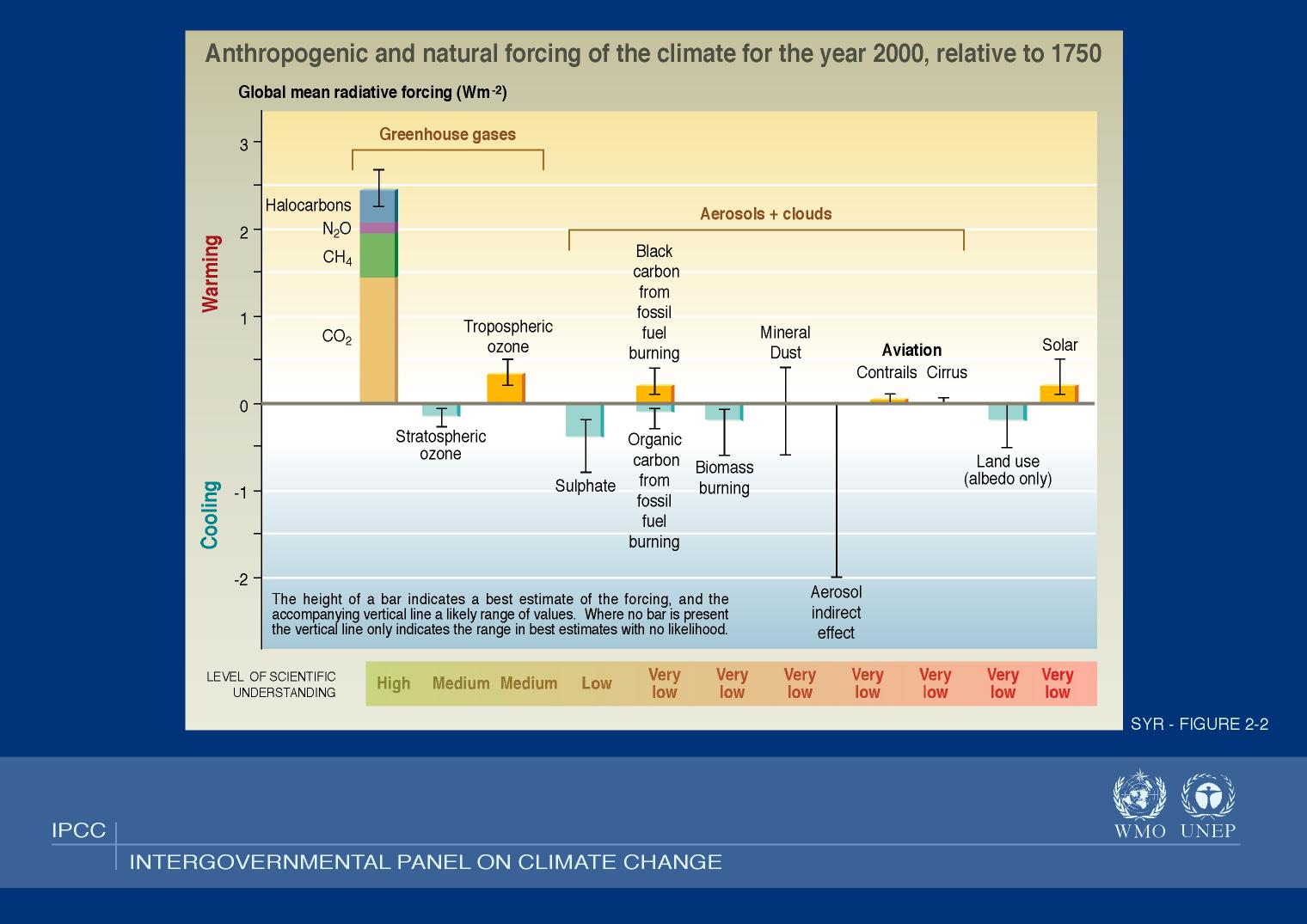
that the pollution cloud was responsible for 50% of the lower atmospheric heating, with the rest attributable to greenhouse gases. The IPCC's 2007 Assessment Report 4 shows that models generally treat aerosols as strongly negative forcings (see adjacent graphic from AR4 Chapter 2, p136).
Note that the uncertainty bars suggest potentially much greater cooling effect but zero potential for atmospheric warming. Adding complexity to modeling requirements these aerosol clouds have now been shown to warm the atmosphere at least as much as increased carbon dioxide
(telling us that models are excessively sensitive to CO2 forcing) and that they should also cool the surface. That's important: In turn the aerosol observations should strengthen the signature expected of enhanced greenhouse warming with the tropical troposphere warming significantly
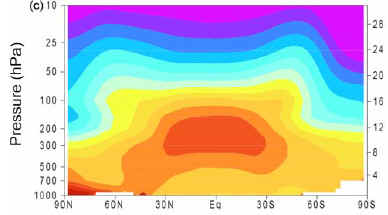
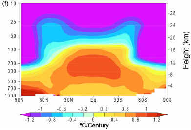
faster than the surface, along with cooling of the stratosphere. AR4 Chapter 9 (p675) offers the following graphical representations, we've imported the greenhouse "bullseye" from the Second-Order Draft simply
because it was conveniently to hand, only differences are cosmetic with the published version being color-enhanced: Caption (from 2nd-order draft): Zonal mean atmospheric temperature change during the 20th century (°C/Century) as simulated by the PCM model from
(a) solar forcing, (b) volcanoes, (c) well-mixed greenhouse gases, (d) tropospheric and stratospheric ozone changes, (e) direct sulphate aerosol forcing, and
(f) the sum of all forcings. Plot is from 1000 hPa to 10 hPa (shown on left scale) and from 0 km to 30 km (shown on right). Based on Santer et al. (2003a). The discovery of such a belt of rapidly warming atmosphere spanning one third of the globe at an altitude of about 20,000' to 50,000' would lend great
support to the enhanced greenhouse hypothesis but has not been found despite diligent searching. There might have been a small step warming in the tropical mid-troposphere a few years ago but HadCRU shows far greater surface warming for the period and GISTEMP suggests even more. While there are no certainties in climate science we now have a few clues regarding possible invalid assumptions. If Kiehl and Trenberth did a fair job of untangling and attributing downwelling radiation then we should expect ΔT ≈ 0.1 °C per Wm-2
ΔF. This is virtually identical to the figure derived from Pielke and that of Idso derived from 8 natural experiments. It is also similar to the figure derived
from revising Hansen for probable change in global cloudiness, as is our Stefan-Boltzmann-derived greenhouse value. Arrayed against these we have the numbers 0.3 °C (which is seemingly close but certainly overestimates current warming), 0.4 - 0.7 K and 0.75 ± 0.25 °C
per Wm-2, from the NAS, Huang and Hansen respectively, all apparently derived from paleo-reconstruction analyses. From these derived numbers and modern measures the implication is that climate sensitivity to ΔF <5 Wm-2 is low, perhaps between one-tenth and
one-fifth °C per Wm-2 ΔF while attempts to reconstruct ancient climes and forcings from proxy measures suggest much greater sensitivity. At the extreme end of the scale we have climate models using 1:1 °C per Wm-2 ratios, at least 5 and probably 10 times greater than recent
observations would suggest. Models might be state of the art but that does not make them useful for predicting future climate states or global mean temperature. As near as we can figure, ΔF 1 Wm-2 = ΔT 0.2 ± 0.1 °C, although this probably overstates sensitivity by omitting Earth's
natural negative feedback mechanisms. Observed change occurs with a net sensitivity of 0.1 °C per Wm-2, while theoretical
calculation suggests 0.2 °C per Wm-2. Hypothetical rates derived from paleo-climate estimates range upwards from 0.3 °C per Wm-2
but cannot be reconciled against observed contemporary changes and are considered highly unreliable. Real-world measures suggest moderate to strong negative feedback, currently unnamed and un-quantified, mitigates the Earth's thermal response to additional
radiative forcing from both human activity and natural variation. Justification for amplification factors >2.5 for unmitigated positive feedback mechanisms is not evident in empirical measures. It is not clear whether
any amplification factor should be applied or even what sign any such factor should be. Nor is there evidence to support such large λ values in GCMs. Division of real-world measures continue to exhibit the same surface thermal response derived by Idso for contemporary local, regional and global climate,
for ancient climate under a younger, weaker sun and for Earth's celestial neighbors, Mars and Venus. In the absence of support for amplification factors and in view of their erroneously large λ values it is apparent that the wiggle fitting so far achieved
with climate model output is accidental or that these models contain equally large opposing errors in other portions of their calculations such that a comedy of
errors produce seemingly plausible results in the short-term. In either case no confidence is inspired. On balance of available evidence then the current model-estimated range of warming from a doubling of atmospheric carbon dioxide should probably be reduced
from 1.4 - 5.8 °C to about 0.4 °C to suit observations or ≈ 0.8 °C to accommodate theoretical warming -- and that's including
ΔF of 3.7 Wm-2 from a doubling of pre-Industrial Revolution atmospheric carbon dioxide levels, a figure we suspect is also inflated. The bottom line is that climate models are programmed to overstate potential warming response to enhanced greenhouse forcing by a huge margin. The median
estimate 3.0 °C warming cited by the IPCC for a doubling of atmospheric carbon dioxide is physically implausible. Copyright © 2006 JunkScience.com - All Rights Reserved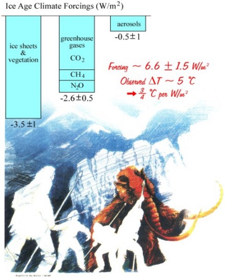 Climate
models usually work on 0.5 - 1.0 °C per Wm-2, which is how they come up with such fantastic warming projections. These numbers are apparently
used based on this estimate by James Hansen: Global climate forcing was about 6 1/2 W/m2 less than in the current interglacial period. This
forcing maintained a planet 5 °C colder than today. (Can we defuse The Global Warming Time Bomb? naturalSCIENCE, August 1, 2003) -- the text
is slightly more specific: "This forcing maintains a global temperature difference of 5 °C, implying a climate sensitivity of 3/4 ± 1/4 °C
per W/m2." The Scientific American version, March 2004, is also available here as 310Kb .pdf.
Climate
models usually work on 0.5 - 1.0 °C per Wm-2, which is how they come up with such fantastic warming projections. These numbers are apparently
used based on this estimate by James Hansen: Global climate forcing was about 6 1/2 W/m2 less than in the current interglacial period. This
forcing maintained a planet 5 °C colder than today. (Can we defuse The Global Warming Time Bomb? naturalSCIENCE, August 1, 2003) -- the text
is slightly more specific: "This forcing maintains a global temperature difference of 5 °C, implying a climate sensitivity of 3/4 ± 1/4 °C
per W/m2." The Scientific American version, March 2004, is also available here as 310Kb .pdf.
 Among the pretty
pictures in "Defusing the global warming time bomb" we find this lovely conceptual image with the caption:
Among the pretty
pictures in "Defusing the global warming time bomb" we find this lovely conceptual image with the caption:
Checking Hansen against the IPCC figures:
Checking Hansen with Stefan's constant:
Sidebar:
How well do we understand radiative forcings?
 Figure 6.6 alt: Figure
6.6 with original caption: Global, annual mean radiative forcings (Wm-2) due to a number of agents for the period from
pre-industrial (1750) to present (late 1990s; about 2000) (numerical values are also listed in Table 6.11 alt: Table 6.11). For detailed explanations see Section 6.13 alt: Section 6.13.
Figure 6.6 alt: Figure
6.6 with original caption: Global, annual mean radiative forcings (Wm-2) due to a number of agents for the period from
pre-industrial (1750) to present (late 1990s; about 2000) (numerical values are also listed in Table 6.11 alt: Table 6.11). For detailed explanations see Section 6.13 alt: Section 6.13.
 (The
"prettier" 06.01 is depicted at right) Apparently we have a high level of scientific understanding only of some greenhouse gases, moderate
understanding of ozone, low of sulfate aerosols and a very low level of scientific understanding of combustion aerosols, mineral dust, indirect aerosol forcing,
aviation-induced contrails and cirrus, land use (changing albedo) and, significantly, solar.
(The
"prettier" 06.01 is depicted at right) Apparently we have a high level of scientific understanding only of some greenhouse gases, moderate
understanding of ozone, low of sulfate aerosols and a very low level of scientific understanding of combustion aerosols, mineral dust, indirect aerosol forcing,
aviation-induced contrails and cirrus, land use (changing albedo) and, significantly, solar.
What do the modelers say?
How do the models perform?
The infamous "smoking gun," from bombshell to bomb...
 The associated media release is entitled
"Earth’s Energy Out of Balance: The Smoking Gun for Global Warming"
The associated media release is entitled
"Earth’s Energy Out of Balance: The Smoking Gun for Global Warming"
 Now Hansen's model has three years of data (minimum) where it's incorrectly
dumping heat into the oceans at a rate of >0.8 Wm-2 when it should not, making it in error over more than 70% of the planet -- call it excess
global forcing of at least 0.56 Wm-2 for that period and thus out by a factor of 3.
Now Hansen's model has three years of data (minimum) where it's incorrectly
dumping heat into the oceans at a rate of >0.8 Wm-2 when it should not, making it in error over more than 70% of the planet -- call it excess
global forcing of at least 0.56 Wm-2 for that period and thus out by a factor of 3.
What if Hansen has misallocated some modern forcings?
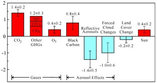 If
we take a slightly more sophisticated approach to net ΔF, (the adjacent graphic is titled "Climate forcing agents in the industrial era (1850–2000)
(W/m2)"), the net change in forcing is shown as ≈ 1.6 Wm-2, which should yield a warming of ≈ 1.2 °C
using the "Hansen Factor", 150-300% of warming believed to have been measured over the period.
If
we take a slightly more sophisticated approach to net ΔF, (the adjacent graphic is titled "Climate forcing agents in the industrial era (1850–2000)
(W/m2)"), the net change in forcing is shown as ≈ 1.6 Wm-2, which should yield a warming of ≈ 1.2 °C
using the "Hansen Factor", 150-300% of warming believed to have been measured over the period.
The "Svensmark Effect":
 With the "two handedness" of economists and researchers everywhere,
there's the possibility both positive and negative forcings are underdone. Recently we had news of important work attempting to quantify
some extraterrestrial influences on Earth's climate, which we featured in Cosmic
Rays and Earth's Climate. This work is particularly interesting in that it indicates positive feedback mechanism for increased solar activity and
negative reinforcement for reduced solar activity, thus explaining how relatively trivial changes in solar activity might equate to ΔF of several Wm-2.
With the "two handedness" of economists and researchers everywhere,
there's the possibility both positive and negative forcings are underdone. Recently we had news of important work attempting to quantify
some extraterrestrial influences on Earth's climate, which we featured in Cosmic
Rays and Earth's Climate. This work is particularly interesting in that it indicates positive feedback mechanism for increased solar activity and
negative reinforcement for reduced solar activity, thus explaining how relatively trivial changes in solar activity might equate to ΔF of several Wm-2.
 There is no
doubt there has been a long-term decrease in Galactic Cosmic Ray (GCR) flux since the late 17th Century, as evidenced by the 10Be and 14C
cosmogenic isotope records (Stuiver and Reimer, 1993; Beer et al., 1994), and this mirrors the long-term increase in Total Solar Irradiance (TSI). In addition,
direct observation shows this increase to be ongoing, see for example, NASA
Study Finds Increasing Solar Trend That Can Change Climate, Solar Irradiance Reconstruction (Lean, 2000) see plot, Sun more active than for a millennium (New Scientist), Sunspots more frequent now than any time for 1000 years (New Scientist), The Sun is More Active Now than Over the Last
8000 Years (Max Planck Society) and so on.
There is no
doubt there has been a long-term decrease in Galactic Cosmic Ray (GCR) flux since the late 17th Century, as evidenced by the 10Be and 14C
cosmogenic isotope records (Stuiver and Reimer, 1993; Beer et al., 1994), and this mirrors the long-term increase in Total Solar Irradiance (TSI). In addition,
direct observation shows this increase to be ongoing, see for example, NASA
Study Finds Increasing Solar Trend That Can Change Climate, Solar Irradiance Reconstruction (Lean, 2000) see plot, Sun more active than for a millennium (New Scientist), Sunspots more frequent now than any time for 1000 years (New Scientist), The Sun is More Active Now than Over the Last
8000 Years (Max Planck Society) and so on.
 Long-term cloud records are in short supply and thus the effect of cloud changes difficult to quantify.
 Obviously a change of roughly 5-10% in cloudiness over just 4 decades is hugely significant although to what extent this is
attributable to local evapo-transpiration and aerosol loading from changes to agriculture, pollutant emissions from rapid expansion of industry and power
generation and exactly what influence changes in GCR flux had over China is as yet unclear.
Obviously a change of roughly 5-10% in cloudiness over just 4 decades is hugely significant although to what extent this is
attributable to local evapo-transpiration and aerosol loading from changes to agriculture, pollutant emissions from rapid expansion of industry and power
generation and exactly what influence changes in GCR flux had over China is as yet unclear.
 On balance it appears solar
forcing, in conjunction with both positive and negative feedback reinforcement according to current trend, might be significantly underestimated in the
attribution of ΔF.
On balance it appears solar
forcing, in conjunction with both positive and negative feedback reinforcement according to current trend, might be significantly underestimated in the
attribution of ΔF.
Update: New data contradicts aerosol cooling hypothesis:
Taking a longer-term perspective using climate-model simulations, Ramanathan's team estimated warming in the lower atmosphere from both aerosols and greenhouse
gases at about 0.25 °C a decade, sufficient to account for the retreat of the Himalayan glaciers. Because the Himalayan glaciers lie at such high
altitudes, they are directly affected by the atmospheric warming effect from brown clouds, yet can also be influenced by soot deposition. Black carbon from
aerosols eventually condenses out of the atmosphere and settles on ice and snow, significantly increasing the amount of sunlight that is absorbed. Researchers
have recently found that the influence of black carbon on temperature and the melting of snow is three times greater than that of CO2 in Arctic
regions. This new information shows us that
aerosol emissions have both heating and cooling effects and, on balance, that aerosols are unlikely to have been 'hiding' anticipated enhanced greenhouse
warming as claimed.
This new information shows us that
aerosol emissions have both heating and cooling effects and, on balance, that aerosols are unlikely to have been 'hiding' anticipated enhanced greenhouse
warming as claimed.

Shaking the mix:
 This is where we commence
arbitrarily hacking at Hansen's table to see if shaking it up a bit results in figures near anything previously derived. Shifting clouds from the negative to
the positive side of the equation would make Hansen's net ΔF ≈ 3.6 Wm-2, which should yield a warming of ≈ 2.7 °C using the
"Hansen Factor," roughly three to seven times the IPCC-estimated value. However, dividing the median estimate of contemporary change (ΔT) of 0.6 °C
by our revised Hansen estimate of 3.6 Wm-2 ΔF, we derive ≈ 0.17 °C per Wm-2, coming back into line with our total
greenhouse divisions performed above. Implied by this newly discovered "consensus" of numbers then is that we have not a good understanding of ΔF
and/or global temperature during a major glaciation since the derived 0.75 °C per Wm-2 appears to be out by a large margin --
"corrected" simply by treating clouds differently.
This is where we commence
arbitrarily hacking at Hansen's table to see if shaking it up a bit results in figures near anything previously derived. Shifting clouds from the negative to
the positive side of the equation would make Hansen's net ΔF ≈ 3.6 Wm-2, which should yield a warming of ≈ 2.7 °C using the
"Hansen Factor," roughly three to seven times the IPCC-estimated value. However, dividing the median estimate of contemporary change (ΔT) of 0.6 °C
by our revised Hansen estimate of 3.6 Wm-2 ΔF, we derive ≈ 0.17 °C per Wm-2, coming back into line with our total
greenhouse divisions performed above. Implied by this newly discovered "consensus" of numbers then is that we have not a good understanding of ΔF
and/or global temperature during a major glaciation since the derived 0.75 °C per Wm-2 appears to be out by a large margin --
"corrected" simply by treating clouds differently.Where does this leave us?
Our best guess at conversion values?
Conclusion: